Vignette#
Generate sankey plot with matplotlib.
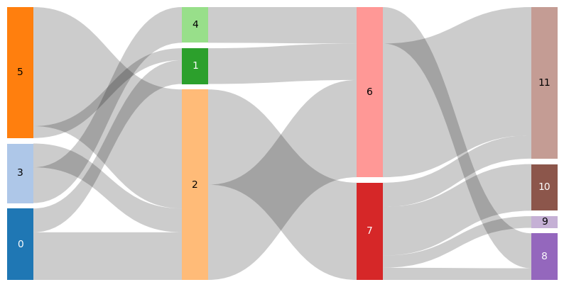
Input data is structured as sequence of sequence of tuple. The tuple contains 3 entries (<source index>, <target index>, <connection weight>).
[1]:
import matplotlib.pyplot as plt
from matplotlib_sankey import sankey, from_matrix
[2]:
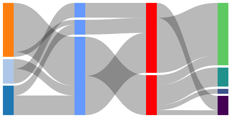
data1 = [
    [(0, 2, 20), (0, 1, 10), (3, 4, 15), (3, 2, 10), (5, 1, 5), (5, 2, 50)],
    [(2, 6, 40), (1, 6, 15), (2, 7, 40), (4, 6, 15)],
    [(7, 8, 5), (7, 9, 5), (7, 10, 20), (7, 11, 10), (6, 11, 55), (6, 8, 15)],
]
[3]:
fig, ax = plt.subplots(figsize=(10, 5))
ax = sankey(
    data=data1,
    color="tab20",
    annotate_columns="index",
    ax=ax,
    spacing=0.02,
)
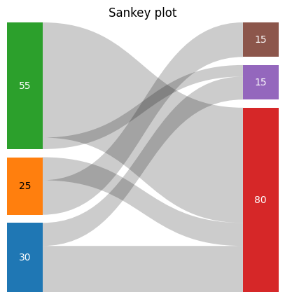
[4]:
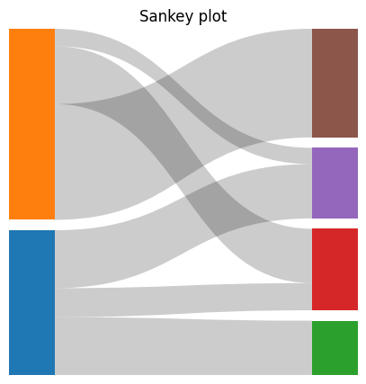
data2 = [(0, 2, 20), (0, 1, 10), (3, 4, 15), (3, 2, 10), (5, 1, 5), (5, 2, 50)]
[5]:
fig, ax = plt.subplots(figsize=(5, 5))
ax = sankey(
    # Sequence arguments must have 3 dimensions
    data=[data2],
    color="tab10",
    annotate_columns="weight",
    ax=ax,
    title="Sankey plot",
    spacing=0.03,
)
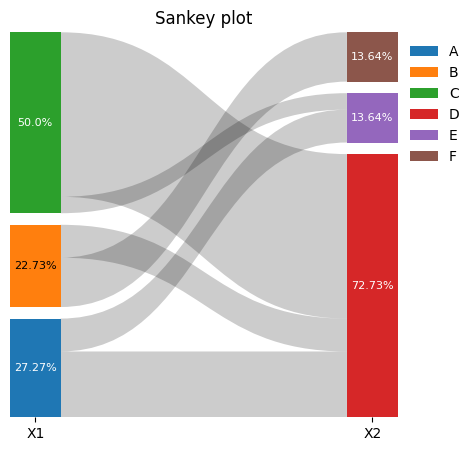
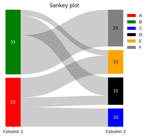
Add legend to plot. Labels of legend handles can be overwritten by legend_labels argument.#
[6]:
fig, ax = plt.subplots(figsize=(5, 5))
ax = sankey(
    data=[data2],
    color="tab10",
    annotate_columns="weight_percent",
    # ax=ax,
    title="Sankey plot",
    spacing=0.03,
    show_legend=True,
    legend_labels=[
        "A",
        "B",
        "C",
        "D",
        "E",
        "F",
    ],
    ax=ax,
    annotate_columns_font_kwargs={
        "fontsize": 8,
        "color": "white",
    },
    column_labels=["X1", "X2"],
)
Color argument also support continous colormap and scales them to number or columns#
[7]:
fig, ax = plt.subplots(figsize=(10, 5))
ax = sankey(
    data=data1,
    color="magma",
    ax=ax,
    spacing=0.02,
    ribbon_color="tab:red",
    ribbon_alpha=0.3,
)

[8]:
fig, ax = plt.subplots(figsize=(10, 5))
ax = sankey(
    data=data1,
    # Column-wise color options
    color=[
        "tab20",
        (0.4, 0.6, 1.0),
        "red",
        "viridis",
    ],
    ax=ax,
    spacing=0.02,
    ribbon_color=(0.1, 0.1, 0.1),
    ribbon_alpha=0.3,
)
Generate input data from connection matrix#
[9]:
data3 = [
    [10, 0, 5, 10],
    [0, 20, 10, 3],
]
[10]:
fig, ax = plt.subplots(figsize=(5, 5))
ax = sankey(
    data=[
        # Optional arguments:
        from_matrix(data3, source_indicies=["A", "B"]),
    ],
    color="tab10",
    # annotate_columns=True,
    title="Sankey plot",
    spacing=0.03,
    ax=ax,
)
[11]:
# Individual definition of colors
fig, ax = plt.subplots(figsize=(5, 5))
sankey(
    data=[from_matrix(data3)],
    color=[
        ["red", "green"],
        ["blue", "black", "orange", "gray"],
    ],
    annotate_columns="weight",
    title="Sankey plot",
    spacing=0.03,
    ax=ax,
    show_legend=True,
    legend_labels=["A", "B", "C", "D", "E", "F"],
    column_labels=["Column 1", "Column 2"],
)
[11]:
<Axes: title={'center': 'Sankey plot'}>
[12]:
from_matrix(
    data3,
    # Optional arguments
    source_indicies=["A", "B"],
    target_indicies=["C", "D", "E", "F"],
)
[12]:
[('A', 'C', 10),
 ('A', 'E', 5),
 ('A', 'F', 10),
 ('B', 'D', 20),
 ('B', 'E', 10),
 ('B', 'F', 3)]
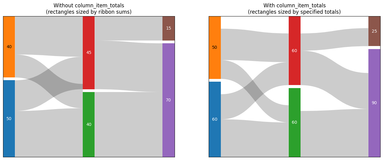
column_item_totals feature.#
When column_item_totals is provided, column items are sized based on these totals rather than just the sum of ribbon weights. This is useful when ribbons only represent a portion of a larger total (e.g., showing flows that are subset of capacity).
[13]:
data = [
    [(0, 1, 30), (0, 2, 20), (3, 1, 15), (3, 2, 25)],
    [(1, 4, 40), (2, 4, 30), (2, 5, 15)],
]

column_item_totals = [
    {0: 60, 3: 50},
    {1: 60, 2: 60},
    {4: 90, 5: 25},
]

fig, (ax1, ax2) = plt.subplots(1, 2, figsize=(16, 6))

sankey(
    data=data,
    ax=ax1,
    spacing=0.02,
    annotate_columns="weight",
    color="tab10",
    show=False,
    frameon=True,
)
ax1.set_title("Without column_item_totals\n(rectangles sized by ribbon sums)")

# Plot with totals
sankey(
    data=data,
    ax=ax2,
    spacing=0.02,
    annotate_columns="weight",
    color="tab10",
    column_item_totals=column_item_totals,
    show=False,
    frameon=True,
)
ax2.set_title("With column_item_totals\n(rectangles sized by specified totals)")
fig
[13]: